· 13 min read
Ethylene with a twist: a chemistry challenge for quantum algorithms
In this post, we'll explore this problem using ethylene (C₂H₄), a simple molecule with a carbon-carbon double bond at its center. How does twisting and bending this double bond change its energy levels?
During a chemical reaction, the bonds that hold a molecule together come under strain. They stretch, bend, twist and contort as reactants transform into products. Being able to predict these transformations is of huge value, from developing new manufacturing processes to discovering new drugs. But doing so means accurately calculating a molecule’s energy in severely distorted configurations. This is where conventional methods of computation struggle, and where quantum computing may offer a promising alternative.
In this post, we’ll explore this problem using ethylene (C₂H₄), a simple molecule with a carbon-carbon double bond at its center. How does twisting and bending this double bond change its energy levels?
We’ll explore two quantum algorithms implemented in OpenQARP, each taking a different approach to the problem:
- Density-of-states quantum phase estimation (DOS-QPE, Scali, Kirsopp et al.), designed for future fault-tolerant quantum computers.
- Quantum computing quantum Monte Carlo (QC-QMC, Buonaiuto et al.), a hybrid quantum–classical method designed with near-term hardware in mind.
We’ll see how each algorithm approaches the problem, compare results and explore what this tells us about the future of quantum chemistry.
Follow along in the accompanying notebook.
Why ethylene, why a double bond? #
Many of the most important chemical processes occur far from a molecule’s natural low-energy structure. As bonds distort in a chemical reaction, electronic states that are normally well separated can move close together or even cross, making their energies much harder to calculate accurately.
This happens throughout chemistry: at the transition states of many thermal reactions, in molecules reacting with a metal catalyst, and in light-driven reactions, where an excited molecule can cross from one state to another before settling to a new equilibrium.
This challenging situation often occurs at double bonds, where two pairs of electrons are shared between atoms. Double bonds are stronger than single bonds and hold the groups at either end rigidly in place. Because of this, the bond will not naturally twist. Making it twist requires partially breaking the bond, for example by heating the molecule, inducing a catalytic reaction, or by absorbing light.
Distorting a double bond is a key step in making plastics, hardening vegetable oils into margarine, and building drug molecules. This is also a crucial process in biology, most famously in your eyes: light twists a double bond in the sensing molecules of your retina to make vision possible.
Ethylene is the smallest molecule with a carbon-carbon double bond. This makes it a standard test case for computing what happens when the bond is distorted. It is also one of the world’s most widely produced organic chemicals, and the starting material for the ubiquitous plastic polyethylene. By twisting and bending ethylene, we can recreate some of the challenging electronic structures that arise in more complex chemical reactions.
Why twisting and bending is difficult #
Energy levels #
The electrons in a molecule can only occupy certain quantum states, each with a particular energy. Together, these form a set of allowed energy levels: the lowest is the ground state, while those above it are excited states. The energy levels move as the atoms move, so chemists picture each one as a landscape over all possible molecular shapes, called a potential energy surface. A reaction is a path across this landscape. Absorbing light excites a molecule from the lowest energy surface onto a higher one, and much of the interesting chemistry happens where two surfaces come close together.
Breaking the double bond #
Ethylene’s equilibrium structure is flat: its six atoms all lie in one plane. The double bond holds the two ends of the molecule aligned, so they cannot twist freely relative to each other. Twisting one end by 90° breaks one of the two shared electron pairs, while the other pair keeps the carbons bonded. The two freed electrons can be arranged in several different ways within the molecule that result in nearly the same energy.
Depending on how their spins are aligned, the electrons can produce different states: a triplet state, in which the two electrons’ spins point the same way and produce three degenerate levels (having exactly the same energy), or a singlet state, in which the spins point in opposite directions and produce a single state. In the calculation we do later, the triplet is the lowest energy state, but the singlet sits only 2.7 mHa above it (mHa stands for milli-hartree, one thousandth of a Hartree, the natural atomic unit of energy). An energy difference of this amount is very small and resolving it requires an extremely accurate calculation.
Where levels touch #
Bending the molecule while it’s twisted brings the energy levels even closer together. If you start from the 90° twisted structure and bend one CH₂ group out of the plane, the two lowest singlet levels move toward each other. When the out-of-plane angle α reaches 68°, our calculation shows that those energy levels meet.
A point where two energy surfaces touch like this is called a conical intersection. It acts as a funnel: a molecule excited by light can drop through it from the upper surface to the lower one, and the direction it leaves in decides what the product of the reaction is. Light-driven reactions like the one in your retina rely on passing through conical intersections.
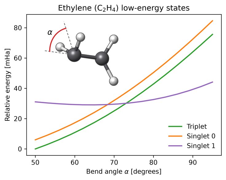
Lowest energy levels of 90°-twisted ethylene against the bend angle α: the triplet and two singlets, with the singlets meeting near 68°. Inset: the twisted ethylene molecule with α marked.
Why classical methods struggle #
On a classical computer, calculating a molecule’s exact energy levels is possible in principle, but the computational cost grows exponentially with the number of electrons involved. Chemists therefore rely on approximations, which work well near a molecule’s equilibrium structure. At distorted geometries like twisted ethylene, however, these approximations are not accurate enough. When energy levels are only a few mHa apart, a small error can put them in the wrong order and predict completely incorrect behavior.
In practice, chemists only need to solve exactly for the handful of electrons involved in the difficult chemistry and can treat the rest approximately. In ethylene, the important electrons are just the pair freed from the broken double bond, so the problem is small enough to solve exactly. In real-world chemical problems, though, it’s more complex. The difficult part can involve dozens of electrons, and the exponential scaling quickly puts an exact classical solution out of reach.
Our calculations focus on these two electrons, requiring just four or six qubits, depending on the model. That is small enough to solve exactly on a laptop, which is deliberate: we can check every result below against an exact answer.
The catch: a quantum algorithm needs a good guess #
Quantum computers are a natural fit for this problem, because qubits can represent every possible arrangement of the electrons at once. The gold-standard quantum algorithm for computing energy levels is quantum phase estimation (QPE). It starts from a trial state, a best guess at the state you want, and returns the energy of one of the molecule’s levels. The closer the trial state is to a given level, the more likely QPE is to return that level’s energy. A good guess at the ground state returns the ground-state energy almost every time; a poor guess returns the wrong level, or needs many repetitions before the right one appears.
The trouble is that good guesses are hardest to make in exactly the situations described above, where energy levels crowd together and no simple guess resembles the right state. This is one of the main open problems for quantum chemistry on quantum computers.
The two algorithms in this post address this challenge with very different approaches. DOS-QPE skips the guess altogether: it probes every energy level at once and returns a histogram of where they lie, the ‘density of states’ in its name. QC-QMC starts from a deliberately rough guess made by a short quantum circuit, then refines it by randomly sampling quantum states built from that guess, steering toward the lowest energy.
DOS-QPE: every level at once #
DOS-QPE works like standard QPE, except for what starting guess is used. Instead of a guess at one state, it starts from an even mix of every possible arrangement of the electrons, so no state is favored over another. Each run then returns the energy of one level, picked at random, and repeating the run many times builds up a histogram with a peak at every level.
Our two electrons in two orbitals can be arranged in six ways, and the molecule has six states to match: the triplet’s three, plus three singlets. Each run is equally likely to land on any of the six, so the triplet, with three states at the same energy, collects half of all runs, and each singlet a sixth. In the figure below, we only show two of the singlet peaks, since the third one is much higher in energy.
How finely the histogram separates energies depends on how many extra qubits (ancillas) are allocated to hold the answer. We use ten, which divide the energy range into 1,024 slots, each about 0.46 mHa wide; levels within about a slot of each other blur into one peak.
In OpenQARP, that is one call:
dosqpe = DOSQPE(unitary, n_ancilla=10, hamming_weight=2,
                engine=QarpEngine(seed=42)).build()
distribution = dosqpe.run()
unitary is a circuit that encodes the molecule’s energy levels,
n_ancilla=10 sets the ten extra qubits, and hamming_weight=2 restricts
the mix to arrangements with exactly two electrons. Each histogram below
collects 10,000 runs on a simulated, noise-free quantum computer.
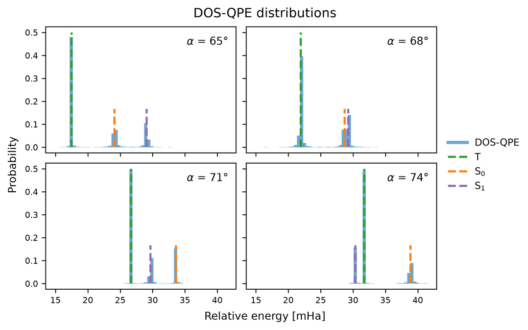
DOS-QPE histograms at four bend angles: three low-lying peaks at 65°, 71° and 74°, with the two singlet peaks merged into one at 68°.
At α = 65°, the triplet and the two singlets give three separate peaks, with the triplet holding half of all runs and each singlet a sixth. (The last sixth goes to the much higher-energy singlet, far off the right of this plot.) The dashed lines mark the exact energies; a peak whose energy falls between two slots is split across both, so it can look shorter than its line. At 68°, the two singlets are 0.6 mHa apart, about one slot, and merge into a single peak: this is the conical intersection. By 71° they have separated again, in the opposite order. Every peak lands within a slot or two of its exact energy, without any guess at the states.
The price for scaling up is circuit size. Each extra qubit of precision doubles the length of the circuit, and with ten, each run repeats the molecule’s circuit about a thousand times. Circuits that long will only run reliably on future error-corrected, fault-tolerant hardware. That makes DOS-QPE an algorithm for machines that have yet to be built, but also one with the clearest route to surpassing what classical computers can do.
QC-QMC: refining a rough guess #
Where DOS-QPE needs long circuits, QC-QMC uses only short ones. It builds on a classical method, quantum Monte Carlo, in which a crowd of random walkers moves among the possible arrangements of the electrons. The walkers spread to connected arrangements, multiply on low-energy ones and “die out” on high-energy ones, and over time the crowd settles into the ground state. Mathematically, these rules carry out a process called imaginary-time evolution, which makes higher energy levels fade away until only the ground state is left. For difficult molecules, simple arrangements of electrons are a poor starting point, and the number of walkers needed grows out of control. QC-QMC replaces those simple arrangements with richer states prepared on a quantum computer.
For this example, we use QC-QMC to follow the ground state as the ethylene molecule is twisted around the double bond, from flat (0°) to perpendicular (90°), in the six-qubit model (two electrons in three orbitals). This is the model in which the singlet sits 2.7 mHa above the triplet at 90°.
The states come from the rough guess: a short quantum circuit with adjustable settings, which a classical computer tunes to lower the energy, a widely used method called the variational quantum eigensolver (VQE). Applying the tuned circuit to the two electrons gives the 15 states the walkers move among, with the guess itself among them.
Because these states are built by a quantum circuit, how strongly each pair is connected has to be measured on the quantum computer. The walkers themselves are tracked on a classical computer, just as in the classical method, and how the crowd is spread across the states gives the energy estimate. We repeat each calculation ten times and average the results.
With the guess circuit in hand, the Monte Carlo run is one call:
mc = MonteCarlo(hamiltonian=qham, approx_ground_state_energy=e_vqe,
                unitary_block=unitary.build(), walker_basis=basis,
                reference_walker_label=bits_to_label(onv),
                initial_walker_count=1000, population_threshold=8000,
                total_time=10.0, time_step=0.1, seed=42).build()
mc.run()
qham describes the molecule’s energy and e_vqe is the energy of the
rough guess. unitary is the tuned guess circuit, basis holds the 15
states built from it, and reference_walker_label marks which of them is
the guess itself. initial_walker_count and population_threshold set how
many walkers start and how large the crowd can grow before its size is
held steady.
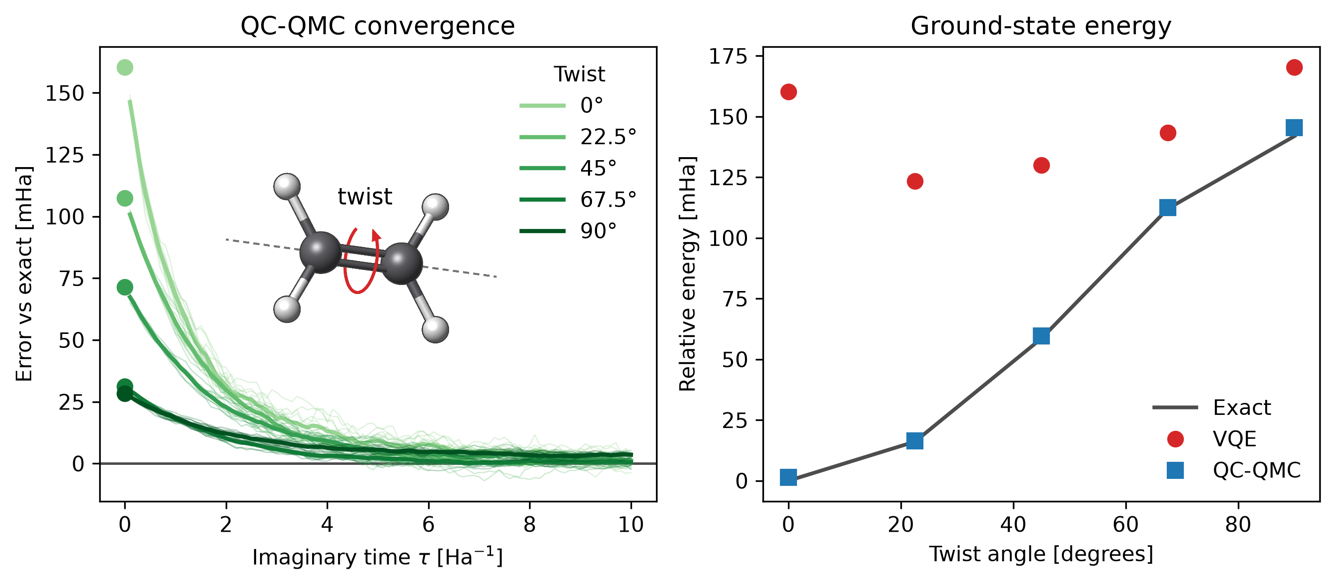
Left: QC-QMC error as a function of imaginary time at each twist angle, starting from the VQE energy. Right: ground-state energy versus twist angle for VQE, QC-QMC, and an exact reference.
The left panel shows QC-QMC at work. Every run starts at the poorly converged VQE energy (the dots) and falls toward the exact answer as the walkers settle in imaginary time. Individual runs scatter by about 2 mHa, some landing slightly below the exact answer. From 0° to 67.5°, the averaged result ends within 1.4 mHa of the exact answer, 60 to 250 times closer than VQE. The right panel collects the final energies and shows the cost of twisting: the ground-state energy rises by 142 mHa from flat to perpendicular, as one of the two shared electron pairs breaks. VQE sits well above the exact curve at every angle, and QC-QMC lies on top of it.
At 90°, where the levels are closest, the runs are still drifting down when they stop, leaving an error of 3.6 mHa, eight times smaller than VQE’s. These are short example runs with loose settings; resolving the 2.7 mHa gap between the triplet and the singlet would need longer runs with more walkers.
What have we learned? #
Distorted molecules are where much of chemistry happens. But they are also where computational predictions get hard. Energy levels crowd together and cross, and the approximations classical methods rely on break down. Quantum computers can represent every arrangement of the electrons at once, but they generally need a good starting guess, and this is harder to make when the molecules are distorted.
The two algorithms we have looked at here take different but complementary routes around this problem. DOS-QPE avoids the need for a guess altogether. It builds a histogram of the different energy levels, counts how many states share each one, and shows when two levels meet at a conical intersection. In contrast, QC-QMC starts from a deliberately rough guess made by a short quantum circuit and lets a random walk do the refining. It cuts the error from tens of mHa or more to about 1 mHa across most of the twist.
Both approaches are promising, but they are designed for different generations of quantum hardware. DOS-QPE requires the long, precise circuits of future fault-tolerant quantum computers. QC-QMC is designed with nearer-term hardware in mind.
Ethylene is a deliberately simple example, but far from an abstract one. It’s an important industrial compound and the behavior of its double bond is relevant to many real-world chemical processes including those involving more complex molecules. At the same time, it is small enough to check every result against an exact calculation.
The real opportunity lies in extending these methods to larger, more complex molecules, where dozens of electrons interact strongly and exact calculations become prohibitively expensive.
Both algorithms are available in OpenQARP, and you can try them yourself. You can explore how they work, reproduce the results and experiment with the parameters in the accompanying notebook.